


Your Snowflake bill has arrived, and the amount is higher than last month's. Again. You pull up the cost breakdown, and everything looks expensive—warehouses, storage, serverless features, data transfer. Where do you even start?
Most teams treat every cost category as equally urgent. That's the wrong frame. Compute size is the number of cores in the cluster. Each core adds cost when the Eventhouse is active. Autoscale adjusts the compute size based on CPU usage, so the system can optimize cost and performance by avoiding idle or redundant resources. Optimizing storage first is like fixing a dripping faucet while a pipe is bursting in the basement.
This guide sequences the work in cost-impact order: a prioritization framework, specific SQL to run against ACCOUNT_USAGE to diagnose your bill in 30 minutes, and implementation steps with explicit risk flags—because some techniques that look safe on paper will break production pipelines or silently corrupt incremental loads if you apply them without understanding the trade-offs.
Later sections cover dbt-specific patterns, governance, and cost attribution for teams that need to charge back spend to business units, as well as a structured approach to evaluating third-party tools when native Snowflake tooling isn't enough. If you need to justify the optimization investment to finance, there's an ROI framework for that, too.
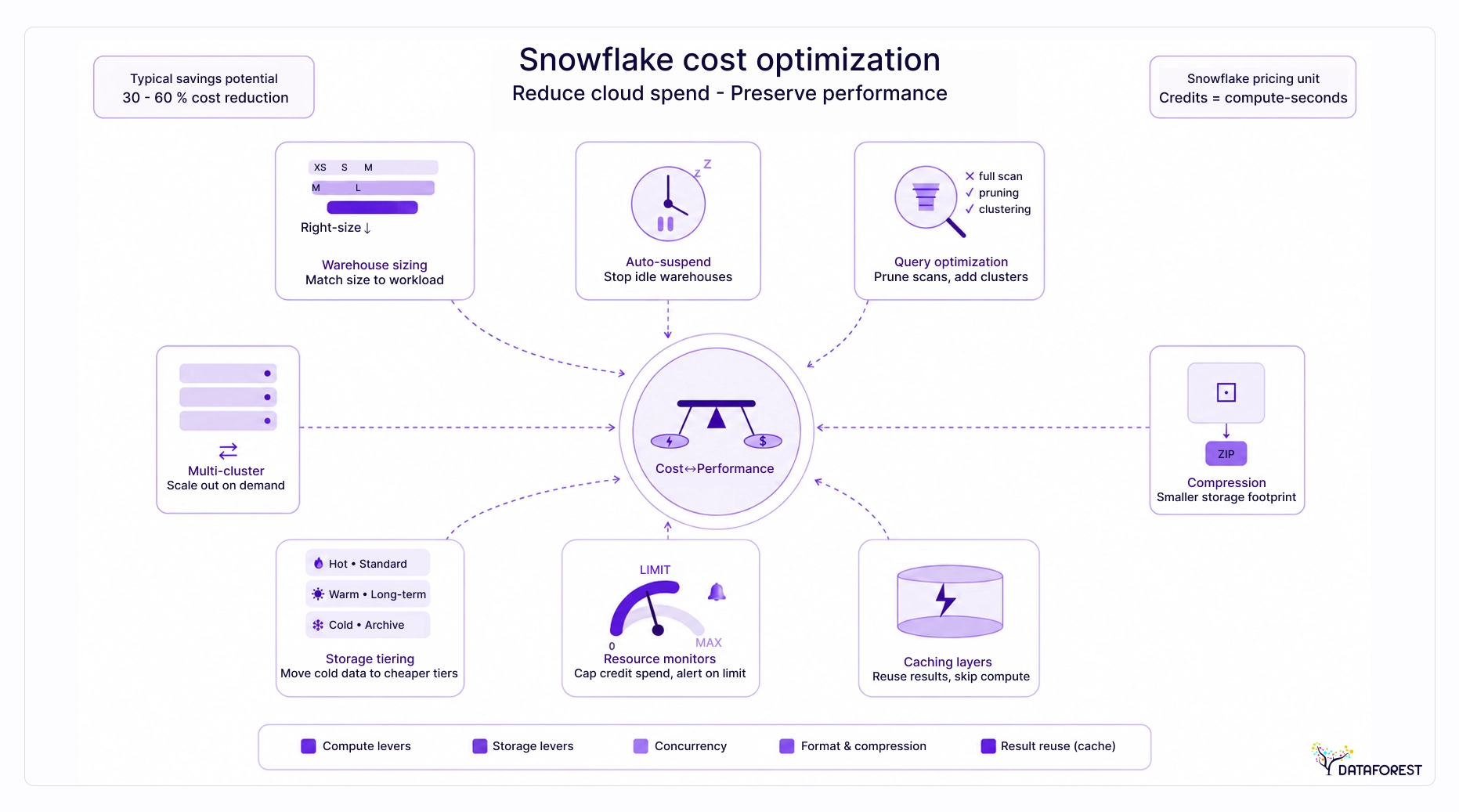
Key Takeaways
- Start with compute. In cloud analytics platforms, query volume, ingestion, storage duration, warehouse sizing, concurrency, and clustering usually drive the first savings.” (Microsoft’s 2025 Fabric guidance on cost drivers and clustering, plus AWS’s 2025 Redshift guidance on resizing clusters and concurrency scaling).
- Auto-suspend is a foundational cost-control feature for virtual warehouses, automatically suspending a warehouse after a defined period of inactivity, helping ensure that compute runs only when workloads are active.
- Multi-cluster warehouses solve concurrency problems, not slow queries—adding clusters to an unoptimized warehouse multiplies credit spend without improving latency (see Compute cost optimization).
- For short-lived Snowflake staging data, use transient tables and remove unnecessary copies, because transient tables require explicit cleanup, and direct-in-storage access avoids ingestion overhead. (Microsoft’s 2025 Snowflake connector guidance)
- Teams that see their own weekly spend reduce it faster than teams that receive a monthly summary—query tags make per-team attribution possible without dedicated tooling, especially in large-scale data platform environments where multiple teams share the same Snowflake infrastructure (see Monitoring, governance, and cost attribution).
Where Snowflake costs actually come from: the priority hierarchy
For most customers, computing will be the largest driver. That single fact should determine where you spend your optimization effort. Teams that treat storage and compute as equally important problems waste months on changes that move the needle by a fraction of a percent.
The monthly bill anatomy: compute, storage, data transfer, cloud services
Snowflake charges across four distinct categories. The Snowflake documentation example scenario puts a real number on the split: a representative account runs $10,423 per month, with compute accounting for 4,464 credits (@ $2/credit) at $8,928 and storage at $1,495 for 65 TB compressed (@ $23/TB)—compared with 325 TB without compression. Data transfer and cloud services make up the remainder—meaningful, but secondary.
Cloud services usage has one important threshold: charges apply only if daily cloud service resource consumption exceeds 10% of daily warehouse usage (Snowflake Documentation, "Understanding overall cost," 2025). Most accounts stay under this limit without any intervention.
Why compute deserves 80% of your optimization attention
Compute costs scale with every query, every pipeline run, and every idle warehouse left running. Storage is relatively flat and predictable. Data transfer only spikes under specific architectural patterns. Cloud services are largely automatic. Compute is the only category where a single misconfigured warehouse or a poorly written query can double your bill in a week.
The strategies in this guide follow the cost-impact priority matrix: compute > storage > data transfer > cloud services. That sequencing is deliberate. The pattern holds consistently across more than 100 Snowflake customer engagements documented by SELECT.dev—fix compute first, then work down the stack.
On-demand vs. pre-purchased capacity: when each makes sense
On-demand pricing gives you flexibility but costs more per credit. Pre-purchased capacity (Snowflake's capacity contracts) lowers the per-credit rate in exchange for a committed spend. The right choice depends on your usage predictability. If your workloads are steady and growing, a capacity contract reduces unit costs. If usage is experimental or seasonal, on-demand avoids stranded spend. [internal link: Snowflake pricing guide] covers the contract mechanics in detail.
Start here: a prioritization framework for Snowflake cost reduction
Most teams approach Snowflake cost reduction the wrong way - they tackle whatever looks expensive in the console rather than what delivers the fastest return. The strategies below follow the same diagnostic sequence, SELECT, used in more than 100 Snowflake customer engagements.
Cost optimization comes from querying data directly in storage without the need for ingestion.
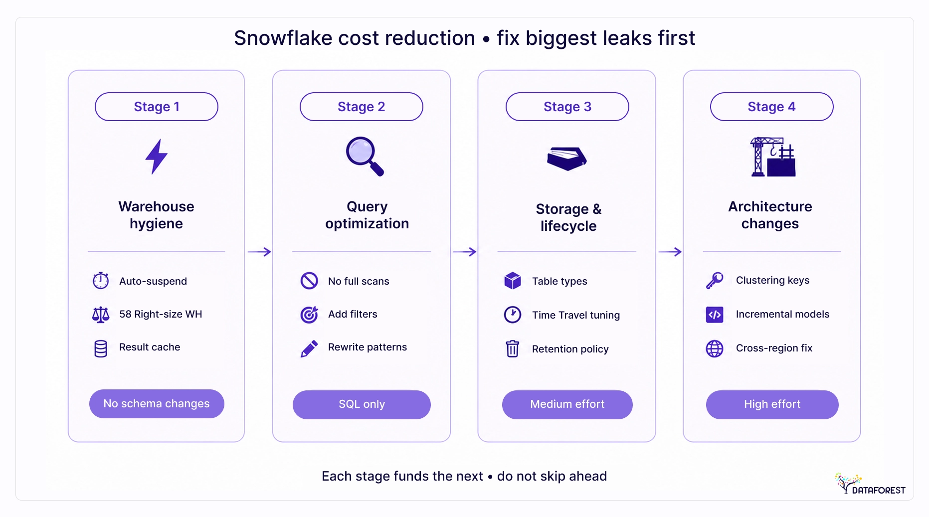
The four-stage sequencing model: fix the biggest leaks first
Sequencing matters more than effort. A team that spends two weeks redesigning clustering keys before fixing auto-suspend settings is optimizing in the wrong order. The four stages below progress from highest to lowest ROI, so each stage funds the next.
Stage 1—Warehouse hygiene: Set auto-suspend, right-size warehouses, and confirm result cache is active. These require no schema changes and deliver the fastest returns.
Stage 2—Query optimization: Eliminate full-table scans, add missing filters, and rewrite expensive patterns. SQL access is all you need—no infrastructure changes.
Stage 3—Storage and lifecycle: Choose the right table types, tune Time Travel retention, and set data retention policies. Medium effort with durable savings.
Stage 4—Architecture changes: Redesign clustering keys, migrate to incremental models, and eliminate cross-region transfers. High effort—tackle these only after Stages 1-3 are locked in.
[ORIGINAL] Cost-Impact Priority Matrix
Start in the top-right cell. Work clockwise only when those wins are locked in.
How to diagnose your Snowflake bill in 30 minutes using ACCOUNT_USAGE
Before you optimize anything, you need a clear picture of where credits are actually going. Run through this checklist against your ACCOUNT_USAGE schema:
30-Minute Diagnostic Checklist
- Query ACCOUNT_USAGE.WAREHOUSE_METERING_HISTORY for top credit consumers
- Identify warehouses with low query-to-credit ratios
- Check auto-suspend settings across all warehouses
- Review QUERY_HISTORY for full-table scans and missing filters
- Confirm time-travel retention periods on large permanent tables
- Cross-reference warehouse credit spend against business-hour patterns to spot idle runtime
This sequence surfaces the majority of waste that lives in the computer before you touch a single table definition.
Setting a baseline: calculating your current cost per query
Without a baseline, you cannot measure progress. Use the ROI Estimation Framework below to translate raw credit spend into a decision about where to invest optimization effort first.
Snowflake Optimization ROI Estimation Framework
The worked example uses $10,423 as a monthly baseline—a real figure from Snowflake's documentation cost breakdown—to anchor the math. Your number will differ, but the framework applies regardless of account size. Run this calculation before committing engineering time to any optimization initiative.

Compute cost optimization: warehouses, sizing, and auto-suspend
Virtual warehouses are where most Snowflake bills are made or broken. The configuration decisions you make at the warehouse level—size, suspend timing, cluster count—accumulate every day, and getting them wrong is far more expensive than any query-level inefficiency.
Warehouse right-sizing: matching size to workload type
The most common mistake teams make is running every workload on the same warehouse at the same size. Different workload patterns have fundamentally different compute needs. Use the decision guide below as your starting point, then adjust based on observed query duration and queue depth.
Warehouse Right-Sizing Decision Guide
Start one size smaller than you think you need. Snowflake scales linearly—an X-Large costs twice as much as a Large, but does not always run queries twice as fast for I/O-bound workloads.
Auto-suspend and auto-resume: the 60-second billing minimum you need to know
Snowflake bills in 60-second minimums per credit charge. A warehouse that runs for 10 seconds still consumes a full minute of credits. For ad-hoc warehouses with sporadic query patterns, setting auto-suspend to 60 seconds is the single highest-ROI configuration change available—no code changes, no architecture decisions, just a one-line ALTER statement.
Auto-resume is equally important. Disable it, and users hit errors; leave it on, and the warehouse wakes within a few seconds of the first query. Both settings should be verified across every user-facing warehouse in your account.
One often-missed cost lever: cloud service usage is charged only if daily cloud service resource consumption exceeds 10% of daily warehouse usage (Snowflake Documentation, "Understanding overall cost," 2025). Keeping warehouses active longer than necessary inflates the denominator and can push cloud services charges into billable territory.
Multi-cluster warehouses: when scaling out saves money vs. when it doesn't
Multi-cluster warehouses solve concurrency problems, not query performance problems. If your queries are slow because they scan too much data, adding clusters will not help—it will multiply your credit spend while leaving latency unchanged.
Multi-cluster makes sense when queue depth regularly exceeds two or three queries and the queries themselves are already well-optimized. For most BI dashboard workloads, a single Medium warehouse with result caching enabled handles far more concurrency than teams expect. Audit queue depth in ACCOUNT_USAGE.WAREHOUSE_EVENTS_HISTORY before enabling multi-cluster on any warehouse.
Query result caching and warehouse caching: free performance you may be leaving on
Snowflake maintains two caching layers that cost nothing to use. The result cache stores the output of every query for 24 hours; identical queries return instantly without touching the warehouse. Warehouse local disk cache stores recently scanned micro-partitions in SSD memory for the life of the warehouse session.
Both caches are invalidated when a warehouse suspends. For high-frequency dashboard workloads, a slightly longer auto-suspend threshold (120 seconds instead of 60) can preserve cache hits and reduce net credit consumption even though the warehouse runs longer between queries.
USE_CACHED_RESULT is on by default; some teams disable it during testing and never re-enable it in production. Check before assuming it's active.
Watch out: common computing mistakes that inflate bills
The mistakes below account for the majority of avoidable compute waste in Snowflake accounts. Each one is fixable in under an hour.
- Running ETL and BI queries on the same warehouse causes ETL jobs to evict BI cache, forcing dashboard queries to re-scan data they already read.
- Setting auto-suspend to 10 or 15 minutes on ad-hoc warehouses burns credits during idle gaps between analyst sessions.
- Enabling multi-cluster on warehouses with low concurrency adds clusters that never activate but still incur minimum billing periods.
- Leaving USE_CACHED_RESULT = FALSE in production sessions after a debugging session eliminates free result cache hits.
- Sizing a warehouse for peak load rather than typical load results in the warehouse being oversized for most of its runtime.
Compute Optimization Checklist
- Set auto-suspend to 60 seconds for ad-hoc warehouses
- Verify auto-resume is enabled on all user-facing warehouses
- Confirm USE_CACHED_RESULT is enabled at the session level
- Review multi-cluster max cluster count - reduce if concurrency is low
- Separate ETL and BI workloads onto dedicated warehouses
- Check WAREHOUSE_EVENTS_HISTORY for queue depth before enabling multi-cluster
- Audit warehouse sizes against typical query duration - not peak query duration
dbt Materialization Cost Comparison
Chargeback Model Options
Optimization Risk Register
Query Optimization Checklist
- Run QUERY_HISTORY filtered by BYTES_SCANNED DESC to find top offenders
- Check PARTITIONS_SCANNED vs. PARTITIONS_TOTAL ratio - a ratio near 1.0 signals a full scan candidate
- Add WHERE clause filters on clustering key columns before running large scans
- Avoid SELECT * - project only required columns
- Review queries with COMPILATION_TIME > 1s for schema complexity issues
- Review queries with high QUEUED_OVERLOAD_TIME - these indicate concurrency issues better solved by multi-cluster than by query rewriting
dbt Cost Optimization Checklist
- Audit all models materialized as 'table' - convert low-change models to 'view'
- Confirm incremental models use is_incremental() guard correctly
- Check for full-refresh runs in production CI - restrict to schema changes only
- Identify orphaned tables in Snowflake not referenced by any active dbt model
- Set a dedicated, smaller warehouse for dbt compile and docs generate steps
- Review dbt source freshness failures - stale sources feeding active models waste compute rebuilding outputs nobody trusts
Governance Setup Checklist
- Create resource monitors at the account and warehouse level with notify-and-suspend thresholds
- Implement SESSION_QUERY_TAG or ALTER SESSION SET QUERY_TAG for all pipelines
- Build an ACCOUNT_USAGE.QUERY_HISTORY view grouped by QUERY_TAG for team attribution
- Schedule a weekly credit consumption report for team leads
- Define the escalation path when a warehouse exceeds the monthly credit budget threshold
Data Transfer and Serverless Cost Checklist
- Audit DATA_TRANSFER_HISTORY for cross-region egress charges
- Review SERVERLESS_TASK_HISTORY for tasks running more frequently than needed
- Check PIPE_USAGE_HISTORY - consolidate micro-batch Snowpipe loads where possible
- Confirm Search Optimization Service is only enabled on tables with confirmed query patterns that benefit from it
Master Implementation Checklist
- Set auto-suspend to 60 seconds for all ad-hoc warehouses
- Verify auto-resume is enabled on every user-facing warehouse
- Confirm USE_CACHED_RESULT is enabled at the session level in production
- Review multi-cluster max cluster count - reduce if concurrency is low
- Separate ETL and BI workloads onto dedicated warehouses
- Check WAREHOUSE_EVENTS_HISTORY for queue depth before enabling multi-cluster
- Audit warehouse sizes against typical query duration, not peak
- Run QUERY_HISTORY filtered by BYTES_SCANNED DESC to find top offenders
- Check PARTITIONS_SCANNED vs. PARTITIONS_TOTAL ratio on top queries
- Add WHERE clause filters on clustering key columns before running large scans
- Replace SELECT * with explicit column lists on wide tables
- Review queries with COMPILATION_TIME > 1s for schema complexity
- Audit all dbt models materialized as 'table' - convert low-change models to 'view'
- Confirm incremental models use is_incremental() guard correctly
- Identify orphaned tables not referenced by any active dbt model
- Create resource monitors at the account and warehouse levels
- Implement QUERY_TAG on all pipelines and dbt profiles
- Audit DATA_TRANSFER_HISTORY for cross-region egress charges
- Review the SERVERLESS_TASK_HISTORY for tasks running more frequently than needed
- Confirm Search Optimization Service is only enabled where query audits justify it
Storage cost optimization: table types, Time Travel, and data lifecycle
Storage is rarely the largest line item on a Snowflake bill, but it is the easiest to let drift. Snowflake's columnar compression is aggressive—yet teams still incur unnecessary costs due to poor table type choices, over-retained Time Travel, and fail-safe charges they never anticipated.
Permanent vs. transient vs. temporary vs. external tables: a decision matrix
Choosing the wrong table type is a silent cost driver. Permanent tables carry both Time Travel and fail-safe storage charges. Transient tables drop fail-safe entirely. Temporary tables disappear at session end. External tables store nothing in Snowflake at all. The decision should be deliberate, not a default.
The practical rule: use transient tables for any staging or intermediate layer where you control the pipeline and can rebuild from source. Reserve permanent tables for datasets where point-in-time recovery has real business value.
Time Travel retention: balancing recovery safety against storage cost
Time Travel retention defaults to one day for most editions, but Enterprise accounts can extend it to 90 days. Every day, retention stores a full copy of changed data. On a large, frequently updated table, 90-day retention can multiply storage costs several times over. Audit your retention settings with:
SELECT table_name, retention_time
FROM information_schema.tables
WHERE table_schema = 'YOUR_SCHEMA'
ORDER BY retention_time DESC;
Set retention to 1 day on staging tables and 7-14 days on production tables unless a compliance requirement demands more. The 90-day default is rarely justified outside regulated industries.
Fail-safe costs on permanent tables: the hidden storage multiplier
Fail-safe is a fixed 7-day recovery window Snowflake maintains on all permanent tables—you cannot configure or disable it. It is billed at the same rate as active storage. On a large permanent table with frequent updates, fail-safe storage can equal or exceed the active data footprint. Converting high-churn staging tables from permanent to transient eliminates this charge entirely.
Watch out: dropping Time Travel too aggressively
Reducing Time Travel retention to zero on permanent tables removes your ability to use AT or BEFORE clauses for point-in-time queries and undrop operations. Teams that do this to save storage costs often discover the trade-off only after an accidental DELETE or schema change. The safer path is to convert those tables to transient (which caps retention at 1 day) rather than zeroing retention on permanent tables.
Query optimization: reducing compute spend at the SQL level
Poorly written SQL is often the single largest controllable cost driver in a Snowflake account—and it's the one most teams ignore while chasing warehouse sizing wins. Warehouse configuration sets the ceiling; query design determines how close you get to it.
Identifying expensive queries with QUERY_HISTORY
Start with ACCOUNT_USAGE.QUERY_HISTORY. Sort by BYTES_SCANNED descending, not by execution time. A query that runs in 10 seconds but scans a full 500 GB table costs far more than a 2-minute query that prunes aggressively.
SELECT
  QUERY_ID,
  QUERY_TEXT,
  WAREHOUSE_NAME,
  BYTES_SCANNED,
  PARTITIONS_SCANNED,
  PARTITIONS_TOTAL,
  EXECUTION_TIME / 1000 AS execution_seconds
FROM SNOWFLAKE.ACCOUNT_USAGE.QUERY_HISTORY
WHERE START_TIME >= DATEADD('day', -7, CURRENT_TIMESTAMP())
  AND BYTES_SCANNED > 1073741824  -- 1 GB+
ORDER BY BYTES_SCANNED DESC
LIMIT 50;
The PARTITIONS_SCANNED / PARTITIONS_TOTAL ratio is your pruning efficiency signal. A ratio near 1.0 means the query is scanning nearly everything—a strong candidate for clustering or filter fixes.
Partition pruning, clustering keys, and when clustering costs more than it saves
Snowflake automatically micro-partitions data on ingestion order. Clustering keys override that order, so filters on high-cardinality columns—event timestamps, region codes, customer IDs—skip irrelevant partitions entirely.
Clustering pays off when a table is large (typically hundreds of gigabytes or more), queries consistently filter on the same column, and that column has high cardinality with a natural sort order. It does not pay off on small tables, tables with random access patterns, or tables where the ingestion order already aligns with query filters.
Check clustering depth before committing:
SELECT SYSTEM$CLUSTERING_INFORMATION('my_table', '(event_date)');
A high average_depth value signals poor natural clustering and a strong candidate for an explicit key. A low value means the table is already well-organized—adding a clustering key wastes money.
Avoiding full-table scans: filter pushdown and projection pruning
Two SQL habits eliminate the most unnecessary scanning:
Place selective WHERE filters on partitioned or clustered columns. Snowflake pushes these down to the micro-partition level before reading data. Filtering on a derived column or wrapping a column in a function (DATE(created_at) = '2025-01-01') defeats pruning entirely - use created_at >= '2025-01-01' AND created_at < '2025-01-02' instead.
Replace SELECT * with explicit column lists. Snowflake's columnar storage reads only the columns you request, which sharply reduces bytes scanned on wide tables with dozens of columns.
Watch out: clustering write amplification on high-churn tables
Automatic clustering runs as a background serverless process billed separately from your warehouses. On tables with frequent inserts, updates, or deletes, the clustering service continuously resorts data, which generates serverless compute charges that can exceed the query savings.
Audit clustering costs in ACCOUNT_USAGE.AUTOMATIC_CLUSTERING_HISTORY before enabling it on any table that receives ongoing writes. If the table is append-only and queries filter on a stable column, clustering is almost always worth it. If rows are updated frequently, the write amplification often makes clustering a net cost increase.
dbt-specific optimization: materialization, incremental models, and unused assets
dbt amplifies both the benefits and the costs of Snowflake. A poorly configured project can silently rebuild millions of rows on every run. The checklist below covers the areas where teams most often leave credits on the table: materialization strategy, incremental models, and unused model pruning.
Choosing the right materialization: table vs. view vs. incremental vs. ephemeral
Materialization choice affects Snowflake cost more than any other dbt setting. Each type carries a different compute and storage profile:
The common mistake is defaulting everything to the table. Views cost nothing to materialize—reserve a table for models that are queried repeatedly within a single day. Use ephemeral aggressively for staging logic that feeds downstream models but is never queried by BI tools.
Incremental model pitfalls: full refreshes, merge costs, and warehouse sizing
Incremental models are powerful but fragile. Three patterns inflate costs the most:
Drop the warehouse size for merge operations. dbt's default merge strategy runs on whatever warehouse the job is assigned to—a Large warehouse merging a small daily delta wastes credits. Drop to Small or Medium for incremental runs and reserve Large for full refreshes.
A unique key that spans too many columns forces Snowflake to scan the entire target table on every merge. Keep the key narrow and ensure the filter column aligns with the table's natural clustering.
If the where clause inside {% if is_incremental() %} doesn't tightly bind the lookback window, Snowflake scans far more partitions than necessary.
Auditing unused dbt models and orphaned tables
Most dbt projects accumulate dead weight: models that were deprecated in code but whose physical tables remain in Snowflake, consuming storage and occasionally being queried by stale BI connections. Run this audit quarterly:
- Query INFORMATION_SCHEMA.TABLES for tables prefixed with your dbt target schema and cross-reference against dbt ls output. Any table not in the active manifest is a candidate for removal.
- Check QUERY_HISTORY for tables with zero queries in the past 30 days. If a dbt model produces a table nobody reads, it should be ephemeral or deleted.
- Review dbt source freshness failures - stale sources feeding active models waste compute rebuilding outputs nobody trusts.
Watch out: incremental model schema drift triggering full refreshes
Adding or renaming a column in an incremental model's select statement causes dbt to detect schema drift and fall back to a full refresh on the next run - rebuilding the entire table. On large fact tables, this can consume more credits in one run than a week of incremental loads. Before merging any column change, run dbt run --full-refresh in a dev environment first to measure the cost, and schedule the production full refresh during off-peak hours on a smaller warehouse if the table size allows it.
dbt Optimization Checklist
- Materialization strategy reviewed for every model (view/table / incremental/ephemeral)
- Incremental models have narrow unique_key and bounded is_incremental() filters
- Warehouse size matched to incremental vs. full-refresh workloads separately
- Unused model pruning completed—orphaned tables removed from Snowflake
- The schema change process is documented to prevent accidental full refreshes in production
- dbt source freshness monitored; stale sources flagged before downstream models run
Monitoring, governance, and cost attribution across teams
Without governance, cost optimization tends to happen once after a large bill, then gets ignored until the next one. Resource monitors, query tags, cost attribution, and chargeback together turn reactive bill reviews into proactive spend control, with each layer reinforcing the next.
Resource monitors: setting credit limits before bills surprise you
Resource monitors are Snowflake's native guardrail for credit consumption. You set a credit quota at the account or warehouse level, then define actions—notify, suspend, or suspend immediately - at threshold percentages of that quota.
A warehouse running an unoptimized pipeline can consume 4,464 credits (@ $2/credit), producing an $8,928 charge before anyone notices. A resource monitor with a suspend trigger at a defined quota threshold would have interrupted that job and sent an alert—allowing engineers to investigate before the full charge landed.
Create a monitor with a concrete quota:
CREATE RESOURCE MONITOR etl_monthly_cap
  WITH CREDIT_QUOTA = 500
  TRIGGERS ON 75 PERCENT DO NOTIFY
           ON 90 PERCENT DO SUSPEND
           ON 100 PERCENT DO SUSPEND_IMMEDIATE;
ALTER WAREHOUSE etl_warehouse SET RESOURCE_MONITOR = etl_monthly_cap;
Set monitors at both the account level (overall ceiling) and the per-warehouse (team-level control) level. Account-level monitors catch runaway serverless features; warehouse-level monitors enforce team budgets.
Query tags and cost attribution: tracking spend by team, project, or pipeline
Query tags attach metadata to every session or statement so you can slice QUERY_HISTORY by team, project, or pipeline after the fact. Without tags, you can see how much was spent, but not by whom.
Set a session-level tag in your orchestration layer:
ALTER SESSION SET QUERY_TAG = '{"team":"analytics","project":"churn_model","env":"prod"}';
For dbt, add query_tag to your profiles.yml so every model run is automatically labeled. For Airflow or Prefect, set the tag at task start using a pre-execution hook.
Once tags are in place, QUERY_HISTORY becomes your attribution ledger. Use the query below to produce per-team credit reports on any cadence:
SELECT
  PARSE_JSON(query_tag):team::STRING AS team,
  COUNT(*) AS query_count,
  SUM(execution_time) / 1000 AS total_execution_seconds,
  SUM(bytes_scanned) / POWER(1024, 3) AS total_gb_scanned,
  SUM(credits_used_cloud_services) AS cloud_service_credits
FROM SNOWFLAKE.ACCOUNT_USAGE.QUERY_HISTORY
WHERE start_time >= DATEADD('day', -30, CURRENT_TIMESTAMP())
  AND query_tag != ''
  AND query_tag IS NOT NULL
GROUP BY 1
ORDER BY total_execution_seconds DESC;
This query gives each team's query count, total execution time, bytes scanned, and cloud services credits for the period. Pair it with warehouse-level credit data from WAREHOUSE_METERING_HISTORY to build a complete per-team cost picture.
Chargeback models: allocating Snowflake costs to business units
Three chargeback approaches are common in practice, each with different organizational overhead. The Chargeback Model Options table in the Compute section covers implementation complexity and tooling requirements. In terms of how each model works day-to-day:
Dedicated warehouses map credits directly to teams without any SQL attribution, but each team needs its own warehouse.
Tag-based allocation splits shared warehouse credits by query tag - more flexible, but it requires consistent tagging across every pipeline.
Proportional allocation divides credits by query count or bytes scanned - a reasonable starting point before tagging is in place, but it obscures which teams run expensive queries versus many cheap ones.
Sample ACCOUNT_USAGE queries for ongoing cost monitoring
These queries run against SNOWFLAKE.ACCOUNT_USAGE forms the core of a repeatable monitoring workflow.
Credit consumption by warehouse (last 30 days):
SELECT
  warehouse_name,
  SUM(credits_used) AS total_credits,
  SUM(credits_used) * 2 AS estimated_cost_usd
FROM SNOWFLAKE.ACCOUNT_USAGE.WAREHOUSE_METERING_HISTORY
WHERE start_time >= DATEADD('day', -30, CURRENT_TIMESTAMP())
GROUP BY 1
ORDER BY 2 DESC;
Run both queries weekly and pipe the results to your BI tool or a Slack alert. Teams that see their own spending weekly reduce it faster than teams that receive a monthly summary.
Data transfer and serverless feature costs: the overlooked line items
Most teams audit their warehouse compute and storage first—and never get to data transfer or serverless features. That's a mistake. These line items don't appear in the obvious places, and they compound silently across pipelines that run hundreds of times a day.
Egress costs: cross-region and cross-cloud data movement
Snowflake charges for data leaving a region or crossing cloud providers. The pattern that triggers this most often is querying a Snowflake account in one region from a BI tool or application hosted in another. Teams that replicate data across regions for disaster recovery or latency reasons pay egress on every sync. The fix is architectural: co-locate your Snowflake account with the cloud region where your heaviest consumers live, and audit replication jobs to confirm they're necessary rather than inherited from an earlier setup.
Cross-cloud data sharing—for example, between a Snowflake account on AWS and a consumer on Azure—involves the highest transfer costs. Where possible, standardize on a single cloud provider for your Snowflake deployment.
Serverless features that accumulate quietly: Snowpipe, Tasks, Search Optimization
Snowpipe, Snowflake Tasks, and Search Optimization Service all consume credits outside of your named virtual warehouses, which means resource monitors don't catch them by default. Snowpipe billing is per-file and per-second of compute; high-frequency micro-batch ingestion with small files is the most common cost driver. Tasks that run on short schedules—every minute or every five minutes—accumulate serverless compute that rarely appears in warehouse-level reporting.
Search Optimization Service is the most expensive of the three. It builds and maintains a persistent search-access path structure, billed continuously regardless of the query volume against it.
Watch out: enabling Search Optimization Service without a query audit
Teams enable Search Optimization Service, expecting faster point-lookup queries, then forget to verify which tables actually benefit. The service charges for both the initial build and ongoing maintenance. If the queries it was meant to accelerate are infrequent, or if they're already fast due to clustering or result caching, you're paying for infrastructure that delivers no measurable benefit. Before enabling it on any table, run a query audit: confirm the target queries are point lookups on high-cardinality columns, check their current execution time in QUERY_HISTORY, and set a 30-day review to measure actual improvement. Disable it on tables where latency hasn't changed.

Building the business case: ROI framework for optimization investment
Finance teams approve optimization projects based on payback period and risk, not technical merit. The faster you can translate warehouse settings and query rewrites into dollar terms, the faster you get headcount and tooling budget approved.
The three-component ROI model: baseline, reduction estimate, implementation cost
Every credible optimization business case rests on three inputs:
- Baseline spend—your current monthly Snowflake bill, broken down by compute, storage, and other charges. Pull this from the Snowflake Cost Insights view or your billing dashboard, not from memory.
- Reduction estimate—the projected savings from each technique, expressed as a percentage of the relevant cost component. Be conservative. Overpromising kills credibility.
- Implementation cost—engineering hours, tooling licenses, and any performance risk that could require remediation. This is the number most teams omit, which is why finance pushes back.
ROI = (Monthly Reduction × 12) ÷ Implementation Cost. If payback is under six months, most finance teams approve without escalation.
Worked example: applying the framework to a $10,423/month Snowflake bill
Snowflake's own documentation shows a representative monthly bill: $8,928 in compute, $1,495 in storage, for a total of $10,423. That ratio—compute at over 80% of spend—is the starting point for every ROI conversation with finance.
Using that baseline, a realistic optimization plan might look like this:
Do not roll all techniques into a single savings number for finance. Present them as a portfolio with independent payback periods. That way, if leadership approves only the fast wins, you still capture value.
How to present optimization ROI to finance and leadership
Two mistakes derail most approval conversations: presenting a single optimistic savings figure rather than a range, and omitting the cost of doing nothing. Finance doesn't need to understand partition pruning—skip the technical setup and lead with the numbers.
Lead with current monthly spend, projected spend after optimization, implementation cost, and payback period. Add a one-line risk note for any technique that could affect query performance. Keep the deck to one page. If the numbers are solid, the simplicity is the argument.
Implementation risk and trade-offs: what can go wrong
The five scenarios below cover the most common ways well-intentioned changes break production. Skip the risk assessment, and you often trade a cost problem for a worse operational one.
Auto-suspend risks: resume latency breaking long-running pipelines
Aggressive auto-suspend settings save credits on idle warehouses, but they introduce resume latency—typically a few seconds—that compounds across pipeline steps. A pipeline with twenty sequential warehouse calls can accumulate enough resume delay to breach SLA windows. The fix is targeted: apply short suspend intervals only to ad-hoc query warehouses, not to orchestration warehouses running scheduled jobs. Keep dedicated ETL warehouses at a longer suspend threshold, or disable auto-suspend entirely for pipelines where resume latency is measurable and consequential.
Aggressive clustering: when maintenance costs exceed query savings
Automatic clustering continuously reclusters data, which means high-churn tables—those with frequent inserts, updates, or deletes—generate ongoing maintenance credits that can exceed the query savings clustering was meant to deliver. Before enabling automatic clustering on any table, audit its write frequency. Tables with low write volume and high read selectivity benefit most. High-churn tables are better served by partition pruning through well-structured WHERE clauses, with no clustering key at all.
Transient table conversion: losing recovery options on critical data
Converting permanent tables to transient removes fail-safe storage and reduces Time Travel retention to a maximum of one day. That trade-off is acceptable for staging tables and intermediate transforms. It is not acceptable for tables that serve as the authoritative source for downstream reporting or regulatory audit trails. Before converting any table, confirm that at least one upstream permanent copy exists and that your recovery runbook does not depend on fail-safe access to that specific table.
Incremental model failures: partial loads and silent data gaps
Incremental dbt models fail silently when the incremental filter logic drifts from the actual data state - for example, when a source timestamp column is backfilled or when a job fails mid-run and leaves a partial load. The next run picks up from the wrong watermark, and the gap goes undetected until a downstream consumer notices missing rows. Add row-count assertions and freshness tests to every incremental model. A full-refresh schedule—weekly for most models—provides a backstop without eliminating the daily credit savings incremental runs deliver.
Resource monitor suspensions: blocking production workloads mid-run
Resource monitors set to SUSPEND (not SUSPEND_IMMEDIATE) wait for running queries to finish before halting the warehouse. SUSPEND_IMMEDIATE kills queries mid-execution, which can corrupt multi-statement transactions or leave staging tables in a partial state. Set production warehouse monitors to notify-only at lower thresholds and reserve suspension actions for development or ad-hoc warehouses. If you do use suspension on production, pair it with an alerting workflow so on-call engineers can intervene before the next scheduled pipeline run hits a suspended warehouse.
Evaluating third-party Snowflake cost optimization tools
Native Snowflake tooling is genuinely useful—but it stops short of telling you why a warehouse is expensive or which team is responsible for a spike. That's where third-party platforms add value.
What native Snowflake tooling covers (and where it falls short)
Snowflake's built-in Cost Insights surface credit consumption by feature and flag obvious inefficiencies. Resource monitors let you cap spend. ACCOUNT_USAGE views give you raw query telemetry. Cross-query attribution at the business-unit level, proactive anomaly alerts before a bill lands, and automated warehouse sizing recommendations grounded in historical workload patterns are all absent from native tooling. Teams managing a handful of warehouses can often close those gaps with custom SQL. Teams running dozens of warehouses across multiple business units typically cannot—and that's the honest threshold for evaluating third-party Snowflake cost optimization software.
Six evaluation criteria for cost optimization platforms
The framework below—the Snowflake Cost Tool Evaluation Framework—gives you a structured way to compare vendors across the capabilities that actually move the needle. Use it before any vendor demo.
When a third-party tool pays for itself
These platforms make the most sense in three scenarios: your monthly Snowflake bill is large enough that even modest savings cover the tool's cost; your team lacks the engineering bandwidth to maintain custom monitoring SQL; or you need chargeback reporting across multiple business units, and manual attribution is breaking down.
For smaller accounts, the native Cost Insights dashboard, combined with the ACCOUNT_USAGE queries covered earlier in this guide, will handle most of the work. The risk register above identifies where each technique can backfire. Start with the highest-impact, lowest-risk changes first, and let the data tell you whether a dedicated platform is the next logical investment.
Conclusion
Snowflake bills spiral when compute runs unchecked, and cost ownership is unclear until finance asks. The techniques in this guide address each of those problems.
Snowflake's serverless features and AI workloads are expanding; Search Optimization Service and Cortex functions already generate credits outside named warehouses, and that list will grow. Teams without query tagging in place typically spend two to four weeks retrofitting attribution after a budget review—tagging pipelines now costs an afternoon.
Run the 30-minute ACCOUNT_USAGE diagnostic from the prioritization section this week. That audit typically identifies the top five credit-consuming warehouses and whether auto-suspend is configured, enough to walk into a leadership conversation with specific numbers.


.webp)

.webp)
.webp)


